Part I: The Foundation of Visibility — Image Enhancement

Introduction: The Philosophy of Machine Sight

Computer Vision (CV) is the science of translating the chaotic, high-entropy stream of photons hitting a sensor into structured, semantic understanding. Unlike a human brain, which has evolved over millions of years to intuitively grasp depth, context, and object permanence, a computer begins with nothing but a grid of numbers—a matrix of pixel intensities ranging from 0 to 255.

The journey from this raw numerical grid to a system that can “Segment Anything” or drive a vehicle autonomously is one of increasing abstraction. It begins with the physics of signal processing (Enhancement), moves through the mathematics of perspective (Geometry), evolves into the identification of distinct landmarks (Feature Extraction), and culminates in the cognitive emulation of neural networks (Architectures).

This report is structured using a Reverse Engineering methodology. For every topic, we first identify the fundamental Problem (why does the raw data fail us?). We then explore the Concept (the mathematical or logical tool available to us). We detail the Solution (the algorithmic implementation used in industry). Finally, we distill the Wisdom (the nuance, trade-offs, and second-order insights defining expert practice).

---

1.1 The Problem: Entropy and the Imperfect Sensor

Before an image can be understood, it must be visible. In the real world, “visibility” is a mathematical property, not just a subjective one. Raw images suffer from three primary corruptions:

1. Poor Contrast: The distribution of pixel intensities is clustered, meaning the signal-to-noise ratio in critical frequency bands is too low for algorithms to detect edges.

   

   Poor contrast occurs when the histogram of pixel intensities is concentrated in a narrow range (e.g., mostly dark grays 30-80 or bright grays 180-230), rather than utilizing the full 0-255 dynamic range. This compression of intensities means that subtle variations—which define edges, textures, and object boundaries—are lost. For computer vision algorithms that rely on gradient calculations or thresholding, this is catastrophic: the mathematically computed “edge” strength drops below detection thresholds, causing objects to blend together as undifferentiated noise.

   Understand the Importance of Contrast and When to use it as Preprocessing Step. Refer an entire tutorial on how to detect low-contrast images programmatically—before you can enhance what you cannot see, you must first detect if the visibility is compromised.

2. Noise: Sensors introduce Gaussian noise (thermal fluctuations) or Impulse noise (dead pixels), creating high-frequency artifacts that mimic edges.

   

   Noise manifests in various forms—from the grainy speckles of thermal noise to the random bright or dark pixels of impulse noise. Each type of noise requires a different approach to detection and removal. For a deeper exploration into the different kinds of noises in image processing, this comprehensive breakdown offers excellent visual examples.

   Once we understand the noise patterns, we can apply computer vision techniques like Noise Removing Techniques using Computer Vision to restore signal clarity and improve downstream algorithmic performance.

3. Illumination Variance: A single scene may contain blinding sunlight and deep shadows. A global exposure setting will inevitably destroy information in one of these regions.

The goal of enhancement is Signal Restoration: modifying the pixel grid to maximize the distinguishability of features without hallucinating new ones.

---

1.2 Histogram Analytics and Contrast Enhancement

1.2.1 Concept: The Probability of Brightness

To manipulate contrast, we must stop looking at the image as a picture and view it as a probability distribution.

The Histogram is a discrete function h(r_k) = n_k, where r_k is the k-th intensity level and n_k is the number of pixels with that intensity.

The normalized histogram represents the probability density function (PDF) of intensity:

# Probability density function (PDF) of intensity
# p(r_k) = n_k / (M * N)
# where:
#   n_k = number of pixels with intensity r_k
#   M * N = total number of pixels (image dimensions)

def probability_density(n_k, M, N):
    """Calculate probability of intensity level r_k"""
    return n_k / (M * N)

where M × N is the image dimension. Low-contrast images have histograms squeezed into a narrow range. High-contrast images utilize the full dynamic range.

There are several Contrast Enhancement Algorithms we will explore some of the major ones.

---

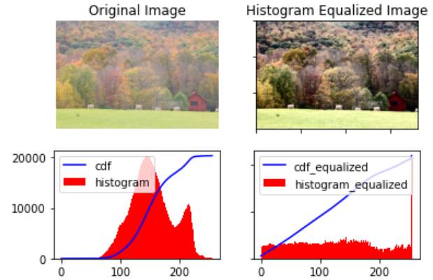
1.2.2 Solution: Global Histogram Equalization (HE)

The most fundamental solution is to flatten the histogram. We seek a transformation T such that the output histogram is uniform (flat).

Mathematically, this transformation is the Cumulative Distribution Function (CDF) of the input.

# Histogram Equalization Transformation
# s_k = T(r_k) = (L - 1) * sum(p_r(r_j)) for j from 0 to k
# where:
#   L = number of gray levels (usually 256)
#   p_r(r_j) = probability of intensity r_j
#   T = transformation function (Cumulative Distribution Function)

def histogram_equalization(r_k, L=256):
    """Transform intensity using CDF"""
    cumulative_sum = sum(p_r(r_j) for j in range(r_k + 1))
    s_k = (L - 1) * cumulative_sum
    return s_k

where L is the number of gray levels (usually 256).

• The Mechanism: This function maps frequent intensities (high probability) to a broader range of the output scale, effectively stretching the contrast where the pixels are most dense.
• The Failure Mode: HE is “Global.” It treats a dark closet and a bright window identically. If an image is mostly dark, HE will stretch the dark pixels across the entire white spectrum. This results in the over-amplification of noise in homogeneous regions (like a clear sky), turning subtle grain into massive artifacts. This Tutorial to Histogram Equalization introduces advanced techniques.

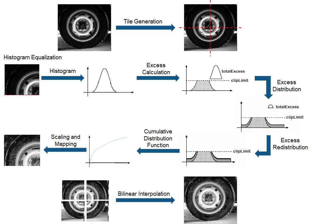
1.2.3 Solution: Contrast Limited Adaptive Histogram Equalization (CLAHE)

To fix the global bias of HE, industry practitioners utilize CLAHE, a technique that processes the image in local tiles.

Algorithm:

1. Tiling: The image is divided into a grid of non-overlapping regions (e.g., 8 × 8 tiles).

2. Local Equalization: The histogram is computed for each tile independently. This allows the algorithm to enhance the contrast of a dark object in a dark corner based only on its immediate neighbors, ignoring the bright window on the other side of the room.

3. Contrast Limiting (The “CL” in CLAHE): This is the critical innovation. In a uniform tile (e.g., a wall), the histogram is a single spike. Standard equalization would take this spike and spread it across the whole range, turning flat wall texture into high-contrast noise.

   • CLAHE introduces a Clip Limit. Any histogram bin above this limit is “clipped.”
   • The excess pixels from the clipped portion are redistributed uniformly across all other bins. This suppresses the noise amplification.5

4. Bilinear Interpolation: If we simply stitched the equalized tiles together, the boundaries would be visible (blocking artifacts). We use bilinear interpolation to blend the results across tile borders, ensuring a smooth gradient.

   

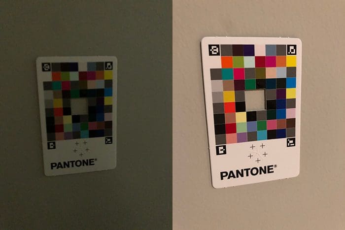
Application Wisdom: Color Space Management

A common mistake is applying CLAHE to the RGB channels of a color image independently. This alters the ratio between Red, Green, and Blue, causing severe color shifting (e.g., a blue sky might turn purple).

• Correct Workflow:
  1. Convert the image from RGB to LAB color space.
  2. Extract the L (Luminance) channel.
  3. Apply CLAHE to the L channel only. The A and B (color) channels remain untouched.
  4. Merge the channels back and convert to RGB. This enhances the details (Luminance) while preserving the original chromatic fidelity.

---

1.3 Denoising Filters: The Battle Against Entropy

1.3.1 The Problem: Signal vs. Noise

Noise is high-frequency variation. Edges are also high-frequency variation. The fundamental challenge of denoising is smoothing out the noise without smoothing out the edges (blurring). lets dive deeper into Image Denoising techniques and challenges

1.3.2 Solution: Gaussian Filtering (Linear)

The Gaussian filter is a weighted average where the weight is determined by the spatial distance from the center pixel.

# Gaussian Filter Formula
# G(x, y) = (1 / (2 * π * σ²)) * exp(-(x² + y²) / (2 * σ²))
# where:
#   σ (sigma) = standard deviation (controls spread/blur)
#   x, y = spatial coordinates relative to center pixel

import numpy as np
import math

def gaussian_filter(x, y, sigma):
    """Calculate Gaussian weight at position (x, y)"""
    coefficient = 1 / (2 * math.pi * sigma ** 2)
    exponent = -(x ** 2 + y ** 2) / (2 * sigma ** 2)
    G = coefficient * math.exp(exponent)
    return G

• Mechanism: It assumes that pixel values change slowly over space. It replaces a pixel with the average of its neighbors.

• Outcome: It is excellent for removing Gaussian Noise (random fluctuations). However, it is a linear low-pass filter, meaning it obliterates high-frequency details like sharp edges. The entire image becomes blurry.

  Explore the difference between Average and Gaussian Filter and the Application of Gaussian Filters as band filters.

  Application Wisdom: The Histogram Hole Phenomenon

  A subtle but critical artifact emerges when applying Gaussian filtering in practice: the creation of artificial “holes” in the image histogram. This occurs due to quantization artifacts during the conversion from floating-point back to integer pixel values.

  

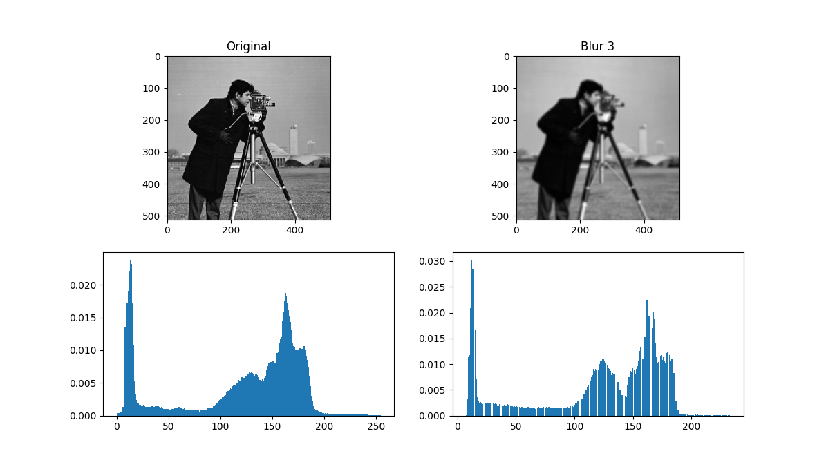
  When you apply a Gaussian filter (which outputs floating-point values) and then round to the nearest integer for uint8 storage, the smoothing operation creates intermediate values that don’t map evenly to discrete intensity bins. Some intensity levels become completely absent from the output histogram, creating gaps that can confuse downstream algorithms like thresholding or histogram-based segmentation.

  This is a well-documented issue in the computer vision community, where practitioners discuss strategies to mitigate this quantization artifact. The solution often involves preserving floating-point precision throughout the pipeline or carefully controlling the filtering parameters to minimize histogram disruption.

1.3.3 Solution: Median Filtering (Non-Linear)

The Median filter comes under spatial filters and is a statistical order - statistical filter. It replaces a pixel with the median value of its neighborhood.

• Mechanism: It sorts the pixel values in the window and picks the middle one.
• Wisdom: This is mathematically superior for Impulse Noise (Salt and Pepper). If a pixel is dead (value 0) or stuck (value 255), it is a statistical outlier. The average (Gaussian) would be pulled significantly by this outlier, smearing it. The median completely ignores the outlier, effectively deleting the noise while preserving the sharp edge of the object.10

Here is Visual Comparison between Median Filter and Gaussian Filter for Salt and Pepper Noise (a) Original Image (b) Image with 10% Noise (c) Result of Median Filter (d) Result of Gaussian Filter

Decision Framework: When to Use Which Filter?

The fundamental difference lies in how these filters handle outliers, and this dictates their optimal use cases.

The Mathematical Difference

• Gaussian Filter computes the mean of the neighborhood: x̄ = (1/n)Σx_i. The mean is highly sensitive to extreme values—a single 255 pixel surrounded by 50s can drag the entire average upward.
• Median Filter computes the median: the middle value after sorting. The median is a robust statistic—it ignores outliers completely.

Gaussian Filter

When to Use It

Use Gaussian filtering when you need to suppress continuous, random noise that follows a normal distribution. This is common in scientific and medical imaging where thermal sensor noise dominates. A mild Gaussian blur is also excellent as a preprocessing step before edge detection or segmentation—it suppresses fine-grained noise that would otherwise create false edges.

In [astronomical image restoration], Gaussian filtering has been essential since the early space program. From the first images of Earth and Moon to modern observations of nebulae and galaxies, Gaussian smoothing reduces sensor thermal noise while preserving the large-scale structure.

When It Fails

Gaussian filtering struggles with salt-and-pepper noise. Because the mean is pulled toward extreme values (0 or 255), isolated noisy pixels create visible “smears” or “ghosts” across the image. Additionally, Gaussian filtering is isotropic—it blurs equally in all directions, which means it will blur across sharp object boundaries, not just within regions of interest.

Median Filter

When to Use It

Median filtering is a go-to choice for impulse noise. Dead pixels in CCD sensors, transmission errors, or “stuck” pixels in cheap cameras—all of these are eliminated effectively because the median ignores outliers entirely. It’s also widely used for preprocessing scanned documents (removing dust speckles while keeping text sharp) and in Synthetic Aperture Radar (SAR) imaging for despeckling.

When It Fails

Median filtering isn’t ideal when noise affects every pixel continuously, as in low-light photography. The median still averages values, but sorted pixel values don’t represent a smooth transition, which can introduce unnatural artifacts. Also, sorting operations are computationally more expensive than Gaussian convolution—for real-time 4K video processing, median filtering may be too slow.

Practical Tip

Many production pipelines combine both filters. For example, apply a median filter first to remove impulse noise, then a mild Gaussian filter to smooth any remaining Gaussian noise before feeding the image to a neural network. This two-stage approach leverages the strengths of both methods.

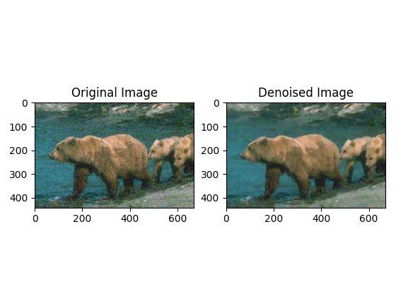
1.3.4 Solution: Bilateral Filtering (Edge-Preserving)

However, the above seen convolutions often result in a loss of important edge information, since they blur out everything, irrespective of it being noise or an edge. To counter this problem, the non-linear bilateral filter was introduced.

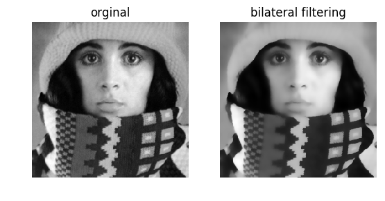
The Bilateral Filter is the standard for “beautification” and high-quality denoising because it is non-linear and edge-aware. It combines two Gaussian weights:

1. Spatial Kernel (W_s): Weights pixels based on geometric distance (like a standard Gaussian).
2. Range Kernel (W_r): Weights pixels based on intensity difference.

# Bilateral Filter Formula
# BF[I]_p = (1 / W_p) * sum(G_σs(||p-q||) * G_σr(|I_p - I_q|) * I_q) for all q in S
# where:
#   W_p = normalization factor
#   G_σs = spatial Gaussian (based on pixel distance ||p-q||)
#   G_σr = range Gaussian (based on intensity difference |I_p - I_q|)
#   S = spatial neighborhood around pixel p

def bilateral_filter(image, p, sigma_s, sigma_r):
    """Apply bilateral filter to pixel p"""
    W_p = 0
    result = 0

    for q in neighborhood_S(p):
        spatial_weight = gaussian_spatial(distance(p, q), sigma_s)
        range_weight = gaussian_range(abs(image[p] - image[q]), sigma_r)
        weight = spatial_weight * range_weight
        W_p += weight
        result += weight * image[q]

    return result / W_p  # Normalize

• The Logic: If a neighbor pixel is close (high Spatial weight) but has a very different color (low Range weight)—indicating it is across an edge—the total weight becomes zero. The filter refuses to average across edges.
• Result: Smooth surfaces (walls, skin) are denoised, but sharp boundaries (edges) remain crisp.

References

• VIDEO: 2D Convolution Explained
• WEBSITE: Interactive Visualisation of Image filters & Kernels
• BLOG: Detect Low Contrast Images
• BLOG: Contrast as Pre-Processing
• BLOG: Different Kinds of Noises in Image Processing
• BLOG: Noise Removing Techniques using Computer Vision
• STACK OVERFLOW: Gaussian Filters Create Holes in Histogram (StackOverflow)
• RESEARCH: Histogram Effects of Gaussian Blurring (ResearchGate)
• VIDEO: Bilateral Filtering in OpenCV Python